PHOENIX Input Data Guide
- James Walker
- Karen Davies (Unlicensed)
This page is under development, please be patient whilst we improve our website. If you have questions that can not be answered by this website at this time please contact us via email: firepredictions@afac.com.au
Overview
Input
When running a simulation Phoenix obtains input data from 3 sources.
- Data entered into the application directly, and saved in the project file,
- Files in the Gridded_Weather directory, and
- Files in the Data directory.
Input data to the model must be prepared in a GIS such as ESRI's ArcGIS or MapInfo. This base data is then converted into a format read by PHOENIX which is an ASCII grid broken into data "tiles", 30 x 30 cells wide. This tiling can be easily done in ArcGIS using a specially developed "Toolbox". The base input data is usually at 20 or 30m resolution, but when it is read into PHOENIX it is averaged into larger cells to speed computations. Typically the grid cell size for PHOENIX computation is 100 or 200m, but could range from 50 to 500m depending on the nature of the terrain and the level of detail required.
This document describes the data files that are obtained from the Gridded_Weather and Data directories.
The actual location of these directories is specified in the project file, and usually defaults to subdirectories of C:\Phoenix
Sub directories :-

The Data Directory
The Data directory normally contains input layers that have been created by hand.
General Requirements
- All data layers must be in the same coordinate system, and this must be a map grid projection (grid reference in metres) not a geographic one (latitude and longitude in degrees).
In Victoria, we suggest using "VicGrid 94" which is a Lambert Conformal Conic Projection with a GDA 94 reference Datum.
Across Australia, we suggest "Geoscience Australia Lambert 94" projection which is a Lambert Conformal Conic Projection with a GDA 94 reference Datum. - The only data layer that MUST be provided is the Fuel Layer.
However, other layers make the simulation much more realistic. If there is no data file location specified, then the input value will be zero. - As all data layers must be in the same coordinate system only one projection file is required. The default name of this file is data.prj and is best located in the root of the Data directory.
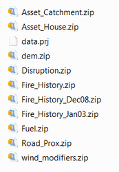
The format of the projection file conforms to the requirements of ESRI ArcGIS 9. - Layers can be provided as zip files, to decrease the size of data that has to be copied around.
Possible Input Layers
The actual layers that Phoenix will use in a simulation are configured in the Project window, on the Data tab. The list below is the complete set of possible layers:
Mandatory
- Fuel Layer - developed from a vegetation layer
Optional
- Digital Elevation Model (DEM) - from which to calculate slope, aspect and elevation
- Fire History Layer, with an optional Supplementary Fire History Layer - from which to calculate the current level of fuels across the landscape
- Road Proximity Layer - from which to determine the level of assistance given to suppression
- Disruption Layer - from which to determine the effect of linear features such as roads, rivers, railway lines and fire breaks, on fire behaviour and spread
- Assets Layer - assists in assessing asset impact during the fire simulation. Assets include Housing, Infrastructure, Plantation and Rainforest
- Wind Modifiers Layer - assists in making changes to local wind speed and direction
- Curing Layer
- Drought Factor Layer
Example :-
Other files in the Data directory
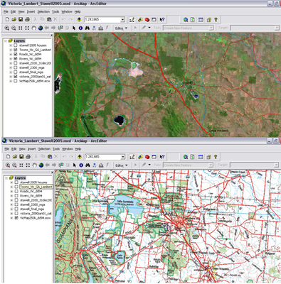
In addition to the source data for running the PHOENIX model, it is also necessary to have a visual reference layer such as a satellite image or topographic map on which to set up the simulation area and to overlay the results of the simulation. More on this below.
This geographic reference layer(s) is encapsulated in an ArcGIS project. Apart from the basic visual reference layer, other GIS information may also be included in this project for display in PHOENIX. However, within PHOENIX, these layers can only be turned on or off for display, no other manipulation of these layers is possible in the PHOENIX environment.
Below are some examples of geographic reference layers. The top image shows a satellite image overlaid with major rivers, roads and town names. The bottom image shows a section of a 1:250,000 topographic map.
Gridded Weather
The Gridded_Weather directory is expected to contain gridded forecast weather data in the form of NetCDF files normally obtained from the Bureau of Meteorology. This data is produced twice a day by the BOM. A downloading process has to be put in place to get this data, but it is restricted to registered users. PHOENIX will also run on a single stream of weather data
TBD - Info about the weather downloader required.
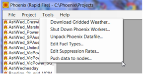
The Tools dropdown menu provides the options to
- Download Gridded Weather - get the latest gridded weather from the Bureau of Meteorology ftp server (only available to registered users)
- Shut Down Phoenix Workers - a facility to run separate simulations, in a parallel process, on a cluster of computers or on different processors for multi-core processors such as Quad-cores. This is a function set up for large simulations.
- Unpack Phoenix Datafile - unpack the zipped input data tiles to compile a single ASCII file
- Edit Fuel Types
- Edit Suppression Rates
- Push data to nodes - such as write the simulation inputs and outputs to the ignition points
TBD - populate this section with a description of how to use the weather downloader
Refer to the manual for how to use weather entered directly into the UI/project file
Other directories
Application
This is where you'll find Phoenix.exe which you can use to run the application.

Outputs
This will ultimately contain the range of files produced from the simulations.
Projects
This will store the .xml files containing the settings for each simulation created.
Data Preparation Requirements
Datum and Coordinate System
All data needs to be prepared in a consistent projection that has a scale in metres. You cannot use a geographic coordinate system using measurement in degrees. For consistency across Australia, we recommend using the GDA_1994_Geoscience_Australia_Lambert projection.
GIS Software
GIS software is an ongoing problem. We have decided to write PHOENIX to use ESRI ArcGIS 9.2, sp4. You need a licence to operate ArcGIS 9.2 ArcView (or similar Arc product such as ArcEditor, ArcInfo). It is our intention to keep the PHOENIX software compatible with the most recent version of ESRI ArcGIS.
Source Data Preparation
1. Fuel (Vegetation)
The Fuel layer is used in conjunction with the fire history layer to create the fuel attributes used in PHOENIX. It has been assumed that the vegetation layer is the layer most likely to be kept up-to-date and more readily available than a purpose built fuel type layer. However, it is also acknowledged that there are several vegetation type classifications and a range of mapping detail and quality within some states and between states. Therefore, the approach taken in PHOENIX has been to convert various vegetation classifications into a standard set of fuel types, e.g. there are about 700 vegetation types mapped in Victoria and these are classified into about 40 different fuel types.
Fuel Types currently recognised in southern Australia.
| Veg Type | FuelCode | No. | Description | Fuel Characteristics |
|---|---|---|---|---|
| Bare | NIL | 0 | Water, sand, no vegetation | fuel absent |
| Herbs | H01 | 30 | Moorland / Fjaeldmarks | low flammability cushion plants |
H02 | 36 | Alpine Herbland | dense, upright, low flammability herbs | |
H03 | 34 | Wet herbland | freshwater herbs on mud flats | |
H03 | 37 | Wet Herbland | low herbs in seasonally inundated lakebeds or wetlands | |
Grass/sedges | G01 | 16 | High Elevation Grassland | dense sward of tussock grasses or herbs, high cover |
G02 | 4 | Moist Sedgeland / Grassland | dense sward, potentially high dead component, button grass | |
G03 | 29 | Ephemeral grass/sedge/herbs | dense grass and sedges with potentially high levels of dead suspended material | |
G04 | 20 | Temperate Grassland / Sedgeland | grasses and sedges widespread, but varying in biomass | |
G05 | 44 | Hummock grassland | hummock grassland, discontinuous surface fuels | |
| Shrubs | S01 | 17 | High Elevation Shrubland/Heath | dense cover of shrubs with surface fuel largely under plants |
S02 | 14 | Riparian shrubland | dense vegetation with little dead material | |
S03 | 35 | Wet Scrub | flammable shrubland with high level of dead elevated fuels | |
S04 | 1 | Moist Shrubland | dense shrubland, salt affected | |
S05 | 31 | Dry Closed Shrubland | tea-tree or paperbark thickets, little understorey | |
S06 | 21 | Broombush / Shrubland / Tea-tree | dense shrubland, but with relatively low level of dead material | |
S07 | 10 | Sparse shrubland | sparse shrubby vegetation with discontinuous surface fuels | |
S08 | 3 | Low flammable Shrubs | low flammability except after exceptional rain bringing grasses | |
S09 | 38 | Mangroves / Aquatic Herbs | trees, shrubs and herbs in permanent water, unburnable | |
| Heaths | S10 | 23 | Wet Heath | dense heath possibly with dense sedgy undergrowth |
S11 | 24 | Dry Heath | dense heath with significant amounts of dead material | |
| Mallee | M01 | 27 | Mallee chenopod | low flammability except after exceptional rain bringing grasses |
M02 | 42 | Mallee grass | mallee woodland with predominantly grass understorey | |
M03 | 25 | Mallee shrub/heath | continuous shrub layer but amount of dead material depending on species present | |
M04 | 26 | Mallee spinifex | discontinuous fuels, very flammable under windy conditions | |
| Woodland | W01 | 18 | High Elevation Woodland shrub | wooded area with shrubby understorey |
W02 | 19 | High Elevation Woodland grass | wooded area with continuous grass tussocks | |
W03 | 97 | Orchard / Vineyard | orchard or vineyard | |
W04 | 2 | Moist Woodland | low trees, shrubby, sedgy understorey, bark hazard | |
W05 | 22 | Woodland bracken/shrubby | wooded area with varying understorey, but not heathy | |
W06 | 9 | Woodland Grass/Herb-rich | surface fuels dominated by grass and herbs | |
W07 | 5 | Woodland Heath | flammable shrubs and high bark hazard | |
W08 | 41 | Gum Woodland heath/shrub | gum woodland with moderate bark hazard, heath/shrub understorey | |
W09 | 43 | Gum Woodland grass/herbs | gum woodland with moderate bark hazard, herbaceous understorey | |
W10 | 39 | Savanna grasslands | tall flammable grasses in an open woodland | |
W11 | 28 | Woodland Callitris/Belah | low flammability except after exceptional rain bringing grasses | |
| Forest | F01 | 15 | Rainforest | dense vegetation with little dead material, epiphytes, vines, ferns, rarely dry |
F02 | 32 | Wet Forest with rainforest understor | ewet sclerophyll forest with mesic understorey | |
F03 | 13 | Riparian Forest shrub | dense vegetation but with a small proportion of dead material | |
F04 | 11 | Wet Forest shrub & wiregrass | high biomass forest, but with little dead suspended material unless wiregrass present | |
F05 | 12 | Damp Forest shrub | dense understorey and potentially high bark hazard (karri) | |
F06 | 40 | Semi-mesic Sclerophyll forest | forest with semi-mesic shurbs and flammable grasses, sedge understorey | |
F07 | 33 | Swamp Forest | dense Melaleuca forest with little understorey | |
F08 | 6 | Forest with shrub | potentially high bark hazard, shrubs moderate flammability (mixed jarrah/karri) | |
F09 | 7 | Forest herb-rich | potentially high bark hazard, little elevated fuel | |
F10 | 45 | Dry Forest shrubs | dry forest with continuous understorey, (southern jarrah) | |
F11 | 8 | Dry Open Forest shrub/herbs | dry forest with open understorey (northern jarrah) | |
| Plantations | P01 | 98 | Softwood Plantation | dense canopy with continuous surface fuels |
P02 | 99 | Hardwood Plantation | uniform canopy with continuous surface fuels |
The user needs to assign a fuel type to every vegetation type in the area of interest. To enable this, a code for each vegetation type is needed, e.g. 97 – Semi-arid Woodland. This code is used in a lookup table and joined to a fuel-type code. This fuel type code must then be added to the attribute table for the vegetation map in a GIS. The setting up of the conversion process is beyond the scope of these notes, but
it can be done by “Joining” the lookup table to the vegetation attribute table in the GIS.
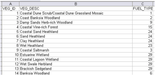
An example of a list of vegetation codes and their matching fuel type code. Several vegetation types may be in the same fuel type.
The fuel mapping must cover the whole area. Areas with no fuel type mapped will be assumed to carry no fuel and therefore will not carry fire (e.g. a water body).
The fuel type layer (and all other input data layers for PHOENIX) needs to be converted to an ASCII grid (.asc) format. The cell size units must be in metres (m), and the cell size must be in whole numbers. A cell size of 30 m is recommended for vegetation. The ASCII file must be called: “fuel.asc”.
Once the “fuel.asc” file has been prepared, it is processed in PHOENIX to compress the data, divided into tiles, and stored in a folder called: “fuel”. This process will be explained in more detail.
Fuel data preparation process - Manual Method
It is necessary for the user to prepare a comprehensive vegetation data layer for the area to be used. Each vegetation type must be identified with a unique code. Below
shows an example of an attribute table associated with a vegetation layer (shapefile). “VEG_ID” is the unique code that will be used to assign each vegetation type to a fuel
type. Once the vegetation layer has been attributed with the fuel type codes, it can be used to create the ASCII grid layer. The name given to this fuel type field is not critical. Producing an ASCII grid is a two step process with the intermediate process being the production of a raster layer with the ESRI grid format.
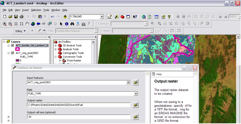
Step 1 - create a unique integer code for each fuel type (ArcMap)

Two tools are available to convert the shapefile to an ESRI GRID (raster), “Feature to Grid” (below) and “Polygon to Grid”. Specify the output file as “vegetation (no extension)” and the output cell size as 30m.
Step 2. Convert the shapefile to an ESRI GRID file. (ARCMap)
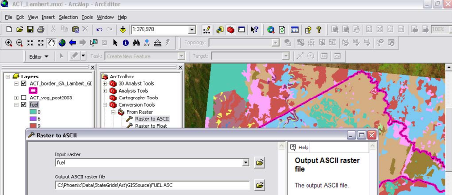
Once the ESRI GRID (raster) file has been created, it must be converted to an ASCII grid format. To do this, use the Conversion Tool – From Raster to ASCII tool. The output ASCII file must be called “fuel.asc”.
Step 3. Convert the ESRI GRID file to an ASCII grid file. (ARCMap)
This ASCII grid file must now be compressed and broken into tiles using a facility in PHOENIX. The fuel, or any other layer, can be converted on its own, or all together, the choice will be yours.
Start by opening PHOENIX. Then select the “Phoenix GIS Data Converter” from the “Data” dropdown menu.
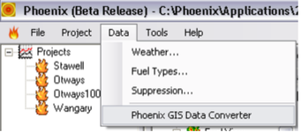
Navigate your way to the folder containing the vegetation ASCII grid file and select it. “Start” the compression and tiling process. The data files will be output to a folder within the one you selected with the ASCII grid file. This folder will be called “fuel” and if it does not already exist, it will be created.
Step 4. Convert the ASCII grid file into a compressed set of ASCII tile files.
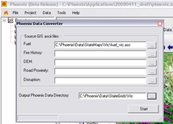
The “Date Converter” tool in PHOENIX converts the ASCII grid data into the format needed to run PHOENIX simulations. Note: in this case only the fuel data is being processed, but other layers could be processed at the same time if desired.
This fuel data will be used in conjunction with the fire history layer to convert them into a current fuel levels when a fire grid is created in PHOENIX. The process of doing this will be explained later.
The fuel layer is now ready for use.
Fuel data preparation process - ArcGIS Toolbox Method
The data preparation process can be simplified by using a set of customised tools developed to be used in ArcGIS 9.2 to produce the data files required as input to PHOENIX.
In order to use these tools, first they must be installed on your GIS program.
Installation
Pre-Check
The toolbox and scripts are stored in a folder in the PHOENIX root directory called Scripts. This will typically be C:\Phoenix\Scripts
It is important to check that these files are in the Scripts folder:
- DEM.py
- Disruption.py
- Fire_History.py
- Phoenix Data Optimiser.exe
- Phoenix.Grid.dll
- PhoenixTools.tbx
- Road_Proximity.py
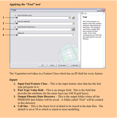
- Fuel.py
The five files denoted with the .py extension are the Python scripts. These are written in Python 2.4 and should work with a standard ArcGIS 9.2 installation.
The .exe and .dll are the files required to perform data conversion from a shapefile or grid format to PHOENIX format. This will be run in the tool, but it is a standalone program that can be run separately on other ASCII files.
The .tbx file is the ArcGIS Toolbox that the user adds to the built-in toolboxes.
Adding the Toolbox to ArcGIS
In this section the user will add the toolbox to the ArcGIS tool list.
Step 1. Open ArcGIS to either the default environment or a previous project.
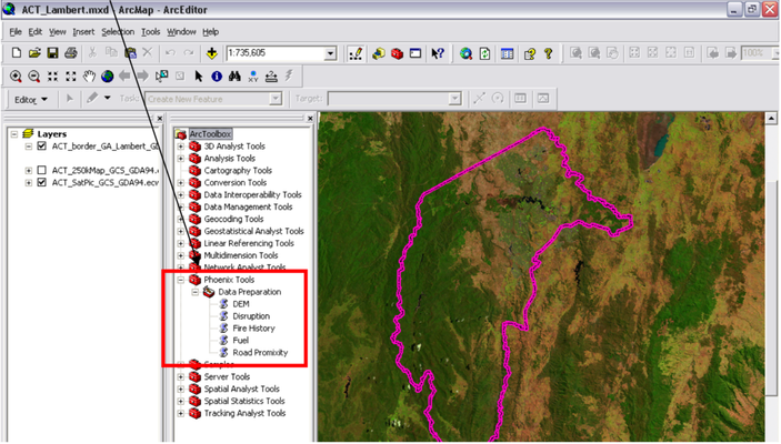
Step 2. Open the toolbox panel by clicking icon 1
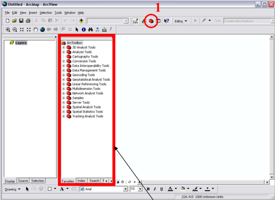
This will open the ArcToolbox panel shown above here
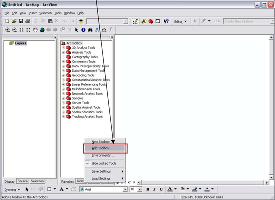
Step 3. Right-click inside the panel so that the context menu opens up and select “Add Toolbox…” as shown below.
Step 4. Navigate to the Phoenix\Scripts directory and select PhoenixTools.
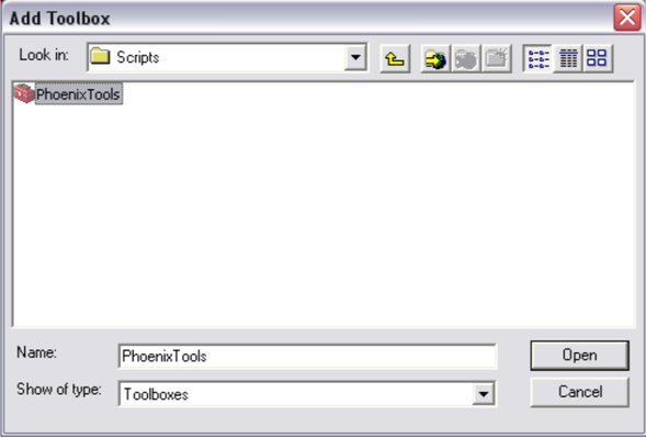
Do not double click as this opens the toolbox as a folder, but doesn’t add it. Once selected, click Open.
Step 5. Once added, click the + next to Phoenix Tools and then the Data Preparation tab and this should expand to reveal the five scripts.
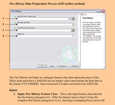
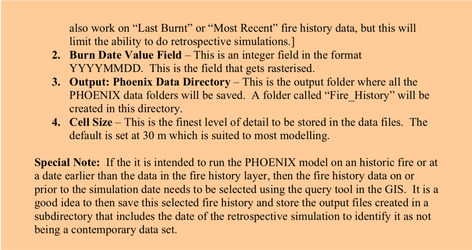
2. Fire History
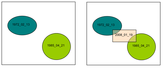
There are two main options for preparing the fire history data layer. The first is to produce a data layer showing the “Last Burnt” fire history where the most recent fire is shown where a previous fire history is replaced by a more recent fire (see below). The second option is where the extent of all known fires is kept, including overlapping fire areas and an effective Last Burnt fire history can be produced for a specified time in the past. This second option has much greater flexibility and is therefore preferred.
The fire history is used in PHOENIX during the fuel layer creation process. Based on the time specified in the simulation, fuel levels will be determined by the combination of fuel type and the time since the last fire.
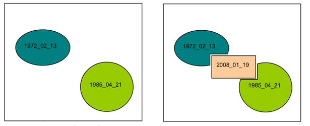
On the left, two fires have been mapped, one in 1972 and the other in 1985. On the right, a new fire in 2008 has overlapped these earlier fires and has replaced their fire history. There is only one layer of fire history.
At present, there is no distinction made between fires of different intensities on fuel accumulation rates. Users should be aware that intense fires that have resulted in structural changes to the vegetation may result in fuel accumulation rates different to those used in PHOENIX.
Fire History Data Preparation Process - Manual Method
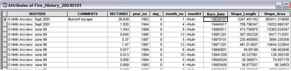
As with the vegetation layer, the aim of this process is to produce an ASCII grid layer containing the fire history information to be used in the simulation. It is recommended that a grid cell resolution of 30m be used. The fire history attribute to be used in the ASCII grid layer is the fire start date MUST be expressed as an integer in the format “YYYYMMDD” (e.g. 19850421). If the actual date is not known then
assume the date to be the 1st January for the season of the fire (e.g. 19850101).
a. Assuming You Have a Current “Last Burn” Layer
Using the GIS, make sure you have a field in the attribute table that contains a fire start date (Burn_Date) expressed as an integer in the format “YYYYMMDD”.
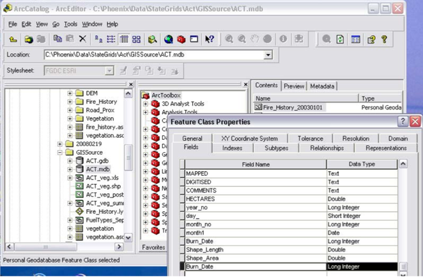
There are a number of ways of creating the Burn_Date. However, first of all, you must create the field in ArcCatalogue. Do this by opening the fire history shapefile and go to the “Fields” tab on the Feature Class Properties and add “Burn_Date” as a long-integer data type. This field MUST be called “Burn_Date”.
Having added the new field “Burn_Date”, you can now either write a Python script to create the data for this field from within ArcGIS, you can use the ArcGIS Field Calculator or you can open the attribute table in MS-Access and fill the fields there. It is always safer to create new fields from within the GIS environment rather than make them in Access, to make sure all the links are maintained.
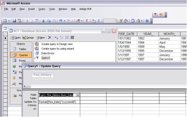
In MS-Access, you can use the Update Query process to convert an existing date (or some other combination) into an integer Burn_Date. One example is shown below.
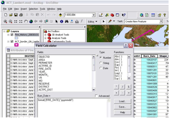
Within ArcGIS you can also create an integer Burn_Date using the Field Calculator, by opening the attribute table, selecting the Burn_Date field and right click to select the Field Calculator window. How you use this calculator will depend on the existing date information in the attribute table already. In the example below, it is just a matter of reformatting an existing date using the “Format( )” function. An alternative approach to achieve the same end is to use the “Data Management Tools”, toolbox and select the “Fields”, “Calculate Fields” option.
- Create a Field in the fire history layer called Burn_Date with an integer date code. (ArcMap)
The following steps are similar to those used in creating the vegetation data. - Convert the fire history layer into an ESRI GRID layer using the Burn_Date as the attribute for gridding. (ArcMap)
- Convert the ESRI GRID file to an ASCII grid file. (ArcMap)
- Convert the ASCII grid file into a compressed set of ASCII tile files.
b. Assuming You Have a Composite (overlapping) Fire History Layer
The first step is to create a Burn_Date field in the fire history layer as described above.
Step 1. Create a Field in the fire history layer called Burn_Date with an integer
In the case of a composite fire history layer, the full extent of all recorded fires is stored in the layer file indicating areas burnt more than once in the recorded history.
Step 2. Convert the fire history layer into an ESRI GRID layer
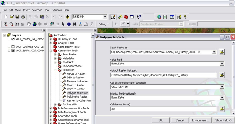
It is necessary this time to use the “Polygon to Raster” Tool. This tool has an option of specifying a “Priority” field. This can be used to specify the “Burn_Date” field so that the most recent (largest) date is used to create the raster layer and all underlying layers (fires) are ignored. In this way, only the most recent fires are recorded for each raster cell.
The remaining two steps are the same as for previous instructions.
Step 3. Convert the ESRI GRID file to an ASCII grid file. (ArcMap)
Step 4. Convert the ASCII grid file into a compressed set of ASCII tile files. (PHOENIX)
The advantage of keeping this overlapping fire history data is that you can create
historic fire history layers for recreation of fire scenarios in the past. Where fires have
overlapped, the most recent fire has not removed the older fire information.
3. Road Proximity Layer
Road Proximity Data Preparation Process - Manual Method
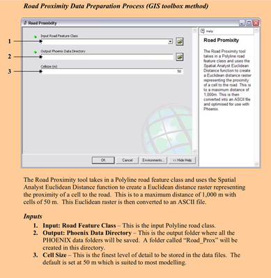
The road proximity layer is used to determine if there is a road within 2000m of a specified point in the landscape, and if it is, how far away it is to the nearest 50m. This information is used in PHOENIX to assess, how much, if any, roads will assist in providing access to fire suppression resources.
In order to develop this layer, first you must have a road layer. This will be a “Polyline” feature layer. Next you will use the Euclidean Distance tool in the Spatial Analyst toolbox to create the Road Proximity layer. The suggested output cell size is 50m and the suggested maximum distance is 1000m. The output file name has to be “Road_Prox”. This is a raster data set.
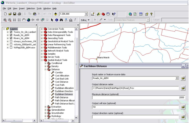
Step 1 (and 2). Create a road proximity layer called “Road_Prox”. (ArcMap)
The following steps are similar to those used in creating the vegetation and fire history datasets. Because the Road_Prox layer is already in ESRI GRID format, Step 2 has already been completed
Step 3. Convert the ESRI GRID file to an ASCII grid file. (ArcMap)
Step 4. Convert the ASCII grid file into a compressed set of ASCII tile files. (PHOENIX)
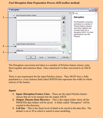
Road Proximity Data Preparation Process - GIS toolbox method
4. Fuel Disruptions Layer
The Fuel Disruption Layer defines the location and width of linear features such as roads, streams, firebreaks, and railway lines which are generally devoid of fuel and may act as barriers to the progress of a fire. There is likely to be a number of GIS layers needed to describe all the linear fuel disruptions in the landscape, however, each of these GIS layers MUST have a field in it called: “WIDTH” which described
the effective width of the fuel-free area along the length of the linear feature (polyline).
The width of the disruption will be used in PHOENIX to determine the extent of the disruptions on the local fire intensity and will determine if the local fire intensity is sufficient to breach the disruption.
Indicative widths of different standards of road, railways and streams as classified by the Australian Standard for GIS mapping AS2482
AS_2482 | Width_(m) | Description |
2000 | 8 | Road in general |
2001 | 12 | Primary Road |
2002 | 60 | Freeway |
2003 | 14 | Highway sealed |
2004 | 14 | Highway unsealed |
2005 | 10 | Main Road sealed |
2006 | 10 | Main Road unsealed |
2007 | 8 | Secondary Road |
2008 | 8 | Secondary Road sealed |
2009 | 8 | Secondary Road unsealed |
2010 | 6 | Minor Road |
2011 | 6 | Minor Road sealed |
2012 | 6 | Minor Road unsealed |
2013 | 4 | Vehicular Track |
2014 | 4 | 4-wheel drive only |
2015 | 5 | Other Roads |
2016 | 5 | Other Roads sealed |
2017 | 5 | Other Roads unsealed |
2018 | 4 | 4-wheel drive only |
2019 | 4 | Road abandoned or under construction |
2030 | 10 | Road, 2 or more lanes, sealed |
2031 | 10 | Road, 2 or more lanes, unsealed |
2032 | 5 | Road, 1 lane, sealed |
2033 | 5 | Road, 1 lane, unsealed |
2034 | 1 | Foot Trail |
2035 | 4 | Mall, Lane, Row, Alley |
2037 | 45 | Divided Highway |
2038 | 30 | Divided Distribution Road |
2039 | 45 | Highway through Built-up Area |
2040 | 8 | Distribution Road |
2041 | 6 | Access Road |
2050 | 10 | Sealed Principal Road for Unrestricted Public Use |
2051 | 10 | Unsealed Principal Road for Unrestricted Public Use |
2052 | 8 | Sealed Secondary Road for Unrestricted Public Use |
2053 | 8 | Unsealed Secondary Road for Unrestricted Public Use |
2054 | 6 | Sealed Minor Road for Unrestricted Public Use |
2055 | 6 | Unsealed Minor Road for Unrestricted Public Use |
2056 | 6 | Sealed Road Public Use may be Restricted |
2057 | 6 | Unsealed Road Public Use may be Restricted |
2058 | 4 | Vehicular Track Public Use may be Restricted |
2059 | 4 | Vehicular Track for Unrestricted Public Use |
2300 | 7 | Railways General |
2301 | 10 | Railways Main Line Commonwealth |
2302 | 7 | Railways Main Line State |
2303 | 7 | Railways Main Line Private |
2304 | 7 | Spur Line, Siding, Yard |
2305 | 3 | Light Railway or Tramway |
2306 | 3 | Disused, Abondoned, Under Construction |
2310 | 7 | Other Lines |
2311 | 10 | Multiple Track Railway |
2312 | 7 | Single Track Railway |
4400 | 8 | General Inland Water Feature |
4404 | 15 | Perennial Watercourse: River, Creek, Stream, Gully |
4405 | 8 | Intermittent Watercourse: River, Creek, Stream, Gully |
4406 | 5 | Mainly Dry Watercourse: River, Creek, Stream, Gully |
4422 | 8 | Watercourse (unclassified) |
4423 | 30 | Braided River (unclassified) |
4424 | 30 | Braided River or Creek, Intermittent |
4425 | 20 | Braided River or Creek, Mainly Dry |
4420 | 15 | Double Line Stream |
4810 | 5 | Channel, Drain, Canal, Ditch, Aquaduct |
Fuel Disruption Data Preparation Process - Manual Method
It is most likely that different disruptive types such as roads, railways and streams will have been mapped in different layers, therefore each layer will need to be prepared and then a combined disruptive layer with a common field “WIDTH” will need to be compiled by appending the files to a master disruptive layer file.
The following instructions assume that the disruptions will be compiled into a raster file, with 30m cells.
Step 1. Create a field in the first disruptive layer called “WIDTH”. (ArcCatalog)
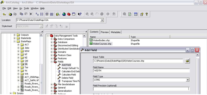
Step 2. Populate the “WIDTH” field.
Use an effective width (m) for each feature using either a lookup table joined to the attribute table of the layer or use the Field Calculator to create a width based on one or other of the attributes in the table.
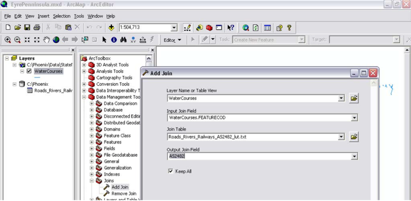
(ArcMap). (Note: step 1 can be omitted if the name of the width field in the join layer is already “WIDTH”.) Join the widths of features to the GIS layer based on a classification of the features such as the AS2482 code.
Step 3. Create a single disruption layer
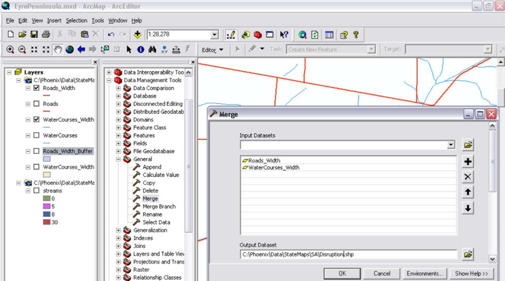
Merge all the disruptive layers into a single layer called “Disruption” using the Merge tool in ArcMap. All files must contain a common field called “WIDTH”.
Step 4. Create a new layer that has a buffer around each polyline.
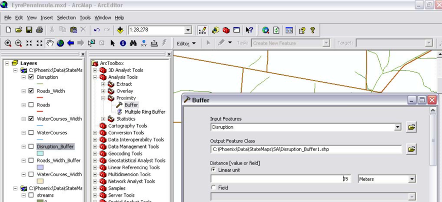
The width of this buffer should equal the size of the raster grid to be used. Use 15m as a default for a 30m raster grid. (ArcMap)
Step 5. Convert the buffered disruptive layer into an ESRI grid. (ArcMap)
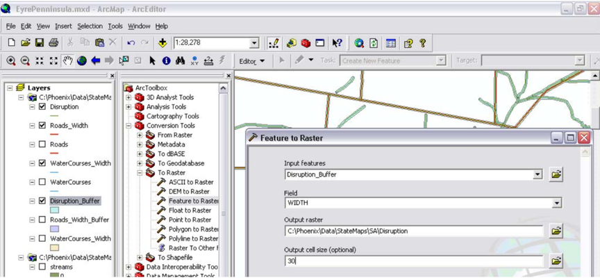
The above show converting the buffered fuel disruptions into an ESRI grid format using the Feature to Raster conversion tool. (see below for an alternative method).
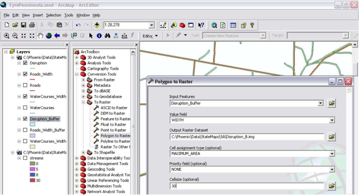
Converting the buffered fuel disruptions into an ESRI grid format using the Polygon to Raster conversion tool. Note that this tool has more options than the feature to raster tool, i.e. the method of picking up polygon attributes (Cell_Centre) and the ability to discriminate which one of a number of overlapping features you will include in the final grid file (Priority Field).
Step 6. Convert the ESRI grid into an ASCII grid. (ArcMap)
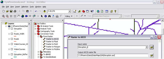
Convert the ESRI grid into an ASCII grid using the Raster to ASCII conversion tool. The output file must be called “disruption.asc”.
Step 7. Convert the ASCII grid file into a compressed set of ASCII tile files. (PHOENIX)
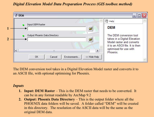
5. Digital Elevation Model Layer
Digital Elevation Model Data Preparation Process - GIS toolbox method
6. Assets Layer
Phoenix incorporates an asset impact model that can calculate asset impact during the fire simulation process. Impacts can calculated for up to 99 asset types and evaluated against up to 99 loss functions, these functions can express loss as a percentage of any of the fire characteristics calculated during the simulation process.
Characterising fires by asset impact provides an additional means of comparing fires. This can be useful for prioritising fires in a tactical scenario or strategically for quantifying the effectiveness of a specific treatment. Asset impact can be a more meaningfully measure than traditional characteristics like fire area, average intensity, perimeter length, etc.
Assets are incorporated as a standard Phoenix dataset. The major limitation of this process is that only one Asset can be recorded against a 30 m cell which requires assets to be in a priority order.
Asset Code Description
The Phoenix asset code is an unsigned 9 digit integer (max integer length supported by shapefile .dbf files). The code is composed of the following 4 parts:
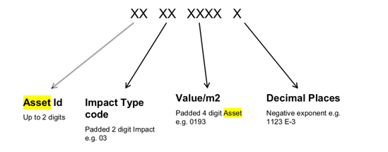
Some worked examples:
| Asset Id | Impact Type Code | Asset Value | Phoenix Integer Scientific Notation | Asset Code |
|---|---|---|---|---|
| 23 | 03 | 1234 | 1234E+0 | 230312340 |
| 11 | 02 | 1.234567 | 1234E-3 | 110212343 |
| 3 | 17 | .0012345 | 0012E-4 | _31700124 |
| 1 | 43 | 50 | 0050E+0 | _14300500 |
Asset Id
The 2-digit asset id is used to report loss against. The current list of assets for Phoenix with their corresponding Impact Types is:
| Asset Id | Description | Impact Type |
|---|---|---|
| 1 | Housing | 2 |
| 2 | Infrastructure | 5 |
| 3 | Plantation | 5 |
| 4 | Catchment Tributaries | 4 |
| 5 | Catchment | 3 |
| 6 | Rainforest | 5 |
Impact Type Code
| Impact Type | Loss Description |
|---|---|
| 1 | Record loss if fire present |
| 2 | HouseLossRatio (Intensity, Ember Density) |
| 3 | Intensity > 3,000 kW/m |
| 4 | Intensity > 10,000 kW/m |
| 5 | Intensity > 30,000 kW/m |
Asset Value
Assets values are all expressed as units per square metre; point assets such as houses will need to be converted to their equivalent density/m2 value. Area based assets such as catchments are given a asset value of 1, indicating a 1 to 1 relationship with burnt area i.e. 1 unit/m2.
Asset values are limited to a maximum of 4 digits and 4 decimal places giving an effective range of .0001 to 9999. Care needs to be taken to ensure suitable units are selected for assets to accommodate this limited range.
Asset Layer Preparation Process
Housing
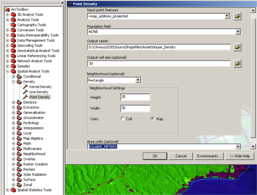
Step 1.
Starting with a house point layer in the correct projection, creates a house point density raster using the ‘Point Density’ tool in the ‘Spatial Analyst Tools – Density’ toolbox. Ensure the settings match the image below, this will create a 3m raster with a per metre housing density value. (Alternatively, Neighbourhood Settings could be 1 x 1 Cells)
NOTE : Ensure 'Area Units' are in m2
Step 2.
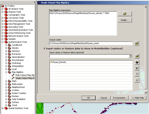
The housing density raster is next converted to a house count raster by multiplying the housing density value by each cells area (30 x 30 = 900m) and add 0.5 to round up. This is done using the ‘Single Output Map Algebra’ tool in the ‘Spatial Analyst Tools – Map Algebra’ toolbox with the following expression:
Int(D:\Otways2030\SourceShapefiles\Asset\house_density * 900 + 0.5)
Step 3.
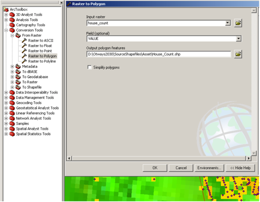
The house count raster is next converted to an intermediate house count polygon shapefile using the ‘Raster to Polygon’ tool in the ‘Conversion Tools – From Raster’ toolbox.
NOTE: Uncheck the 'Simplify polygons' check box
Step 4.
NOTE : Delete all polygons with a house count of 0 after conversion to polygon. This significantly reduced the size of the file and speeds later processing.
Step 5.
Add a ‘House Density’ column (Double Precision) and using the "Calculate Field" option on the source table, convert the house count value back to a metre square density value by dividing the house count by 900.
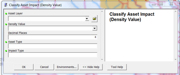
Step 6.
Using the Phoenix asset classification tool for density values, generate the asset code
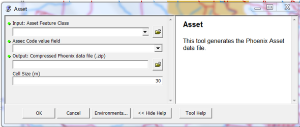
Step 7.
Finally use the Asset tool in Data Preparation toolbox to convert the housing layer into Phoenix Format.
NOTE : Convert to raster doesn’t seem to work from within a file geodatabase, export to shapefile before converting.
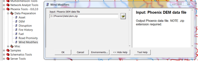
7. Wind Modifiers Layer
The "Wind Modifiers" data layer assists in making changes to local wind speed and direction due to the influences of the topography. Phoenix uses a "Mass Conservation" model called "Wind Ninja" developed by Jason Forthofer in 2007. A mass conservation model allows for winds to speed up over hills and be channeled up valleys to some extent, but it does not reproduce the full fluid dynamics of wind flow. However, it is considered worthwhile to take some account of topography on local wind speed and direction rather than assume that it is uniform across the landscape.
The only input data needed to create the Wind Modifiers layer is the Phoenix DEM (topography) layer. Winds of all speeds and directions are modelled across this terrain to determine the appropriate wind modifiers for all situations.
Use the "Wind Modifiers" tool in the Phoenix Toolbox to create this data layer for Phoenix. The output file will be in the same folder as the DEM layer used. This process can take a very long time.