PHOENIX User Manual
- James Walker
- Karen Davies (Unlicensed)
This page is under development, please be patient whilst we improve our website. If you have questions that can not be answered by this website at this time please contact us via email: firepredictions@afac.com.au
This document will describe how to use Phoenix from a very 'manual labour' standpoint of what buttons do what and what gets entered into each field.
Will refer to separate pages for the installation instructions, how to set up data, etc
Introduction
PHOENIX RapidFire is a fire characterisation model used to capture the nature of a fire as it spreads across the landscape. As it spreads, fire characteristics such as flame height, intensity, size, ember density and captured in a spatial database. It is also designed to capture the impact of the fire on various values and assets in the same spatial database. The impact is based on the interaction of the fire characteristics and the vulnerability of the asset or value to fire, such as fire intensity or ember density. Inputs to the model come from the same spatial database and include fuel type, fire history, slope, aspect, and weather.
Input data to the model must be prepared in a GIS such as ESRI's ArcGIS or MapInfo. This base data is then converted into a format read by PHOENIX which is an ASCII grid broken into data "tiles", 30 x 30 cells wide. This tiling can be easily done in ArcGIS using a specially developed "Toolbox". The base input data is usually at 20 or 30m resolution, but when it is read into PHOENIX it is averaged into larger cells to speed computations. Typically the grid cell size for PHOENIX computation is 100 or 200m, but could range from 50 to 500m depending on the nature of the terrain and the level of detail required.
Set Up
PHOENIX is a standalone application and does not need installation. It can just as easily run from a USB stick as from a computer hard-drive. It is suggested that PHOENIX software and data be placed on the C: drive for ease of setting pathnames, but will work from any location.
Software requirements:
Microsoft.NET framework Version 3 or later (essential)
Google Earth (highly desirable)
ArcGIS or other GIS (necessary to prepare data and analyse outputs)
For input data set up refer to PHOENIX Input Data Guide.
The "Gridded_Weather", "Outputs" and "Projects" sub-folders may be empty until the model has been run. Once run the "Outputs" folder will hold the range of files produced from the simulations. Names of files in this folder will be based on the name of the project the user specifies. The "Projects" folder stores the ".xml" files containing the settings for each simulation created.
For ease of use, it is handy to create a shortcut for PHOENIX on your desktop.

Running a Simulation
Start PHOENIX by running the PHOENIX.exe program located in the "Application" folder. The flash screen will come up displaying the version of PHOENIX you have and warning you of the limitations of the program. You must read these warnings and indicate that in using the program you acknowledge the program limitations.
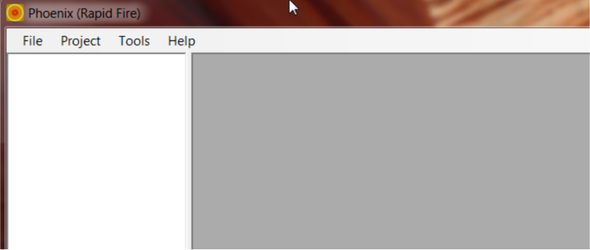
Once you have accepted the conditions of use, the main window will open. The toolbar contains dropdown menus for "File", "Project", "Tools" and "Help". A list of all the existing projects will be shown in the "Projects" file window.
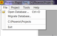
The "File" dropdown menu contains the options of opening an existing database, migrating a database from an earlier version of PHOENIX, finding an existing file in the "Projects" sub-folder, or exiting the program.
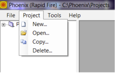
The "Project" dropdown menu contains the options for creating a new project, opening an existing project, creating a new project by copying an existing one, and deleting a project.
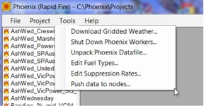
The "Tools" dropdown menu provides the options to download the latest gridded weather from the Bureau of Meteorology ftp server (only available to registered users) and an option to shut down PHOENIX Workers which is a facility to run separate simulations, in a parallel process, on a cluster of computers or on different processors for multi-core processors such as Quad-cores. This is a function set up for large simulations. You can also "Unpack" the zipped input data tiles to compile a single ASCII file, edit the fuel types file, edit the Suppression Rates attributes or "Push data to nodes" such as write the simulation inputs and outputs to the ignition points.
The "Help" menu provides information about this version of the software. There are help speech bubbles that appear when the cursor is held over fields requiring some explanation.
Creating a New Project
A new project can be created by using the "Project" > "New" menu or by copying and modifying an existing project using the "Project" > "Copy" menu.
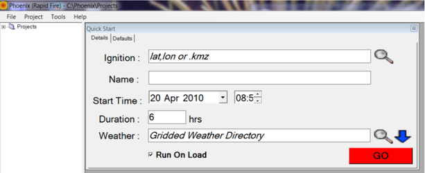
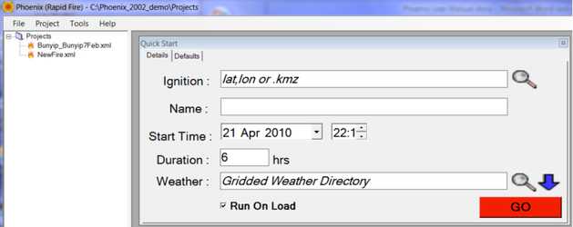
'Quick Start' Project Creation
The "Project" > "New" option will bring up a "Quick Start" window. The new project will need an Ignition location entered as a Latitude/Longitude or as a "kmz" file from a Google Earth place marker. A name will be needed for the project, a start time and date for the fire ignition and the path to the directory containing the gridded weather data.
If you are not using a KMZ file to identify the ignition point, then the latitude and longitude can be
entered in any of the following formats:
37° 21' 55.0" S, 145° 9' 49.6" E (Fireweb)
37°21'54.98"S (google earth default)
37° 21.916'S  (google decimal minutes)
-37.365272°   (google decimal degrees)
Manual Project Creation
An alternative approach is to manually develop a project by copying the "Template.xml" project from the "Application" folder to the "Projects" folder and then edit this.
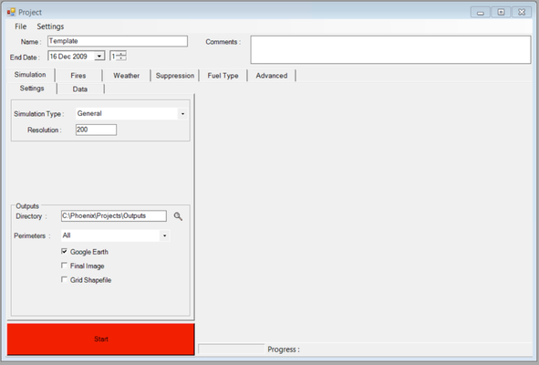
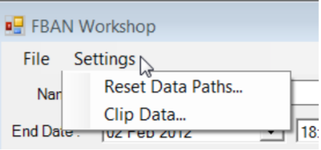
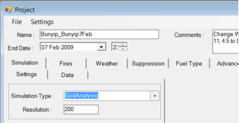
The Project window has two Menu options: "File" and "Settings" and eight (8) window tabs. The "File" menu contains two options - "Save" and "Validate Project". The "Save" option updates the project settings in the project file and the "Validate" option does a quick check for any logical errors or missing information in the project that will prevent it from running. The validation process is automatically run before each simulation, but this menu option allows you to do a quick, pre- simulation check.
The "Settings" menu provides two tools to update the information in the "Settings" tab of the "Simulation" options. The first tool does a global find and replace of the file path to the data folders. The second tool "Clip Data" will compile a composite ASCII file of a specified data layer within the bounds of a nominated shapefile, e.g. you could extract the fire history or fuel data for an area of interest and display it in a GIS.
- Name - enter a name that identifies the project e.g. 'Demo Run'
- End Date - enter the date and time for the end of the fire simulation. If more than one fire is being simulated, they will all end at this same time and date. There are separate windows for the date and time. Note: the end date must fall within the range of the weather data specified.
Simulation → Settings
This is where you specify how the simulation will be run and the type of outputs required (more details of the types of outputs are given later).
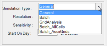
There are six (6) simulation types:
| Simulation Type | Description / Outputs |
|---|---|
| General | This is the simplest mode. All fires listed in "Fires" list will be run simultaneously using the weather and suppression conditions listed in this table. If a folder is listed in the "GFE Weather" tab then the gridded weather data will be used in preference to the weather stream listed in the "Fires" list. Simulation outputs can be specified as any combination of "Perimeters" (isochrones of fire spread), Google Earth animation, PNG image files, and grid shapefile with input and summary output variables. |
| Batch | This will run each fire independently (a discrete event). The output from this simulation will be the Fire Impact CSV file and a Scenario table. 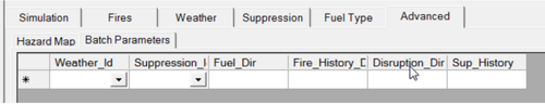 |
| Grid Analysis | Also produces the Fire Impact CSV file and Scenario table, but also a Cell Impact CSV and Ascii grid with all the cumulative values for each cell and PNG images of the main summary statistics such as Asset Impact, Burn Frequency, Ember Density, Flame Height, Intensity, and House Loss. |
| Batch All Cells | As for Grid Analysis but also includes a table (CSV) with values of fire attributes for each cell for each fire so there can be multiple records per cell ("AllCells"). |
| Batch Ascii Grids | As for "Grid Analysis" but the output for each fire (Ascii grid of Flame Height and Intensity) is kept separately. This generates a lot of files and output data. |
| Automate Risk | Automates the statewide daily risk analysis. |
If one of the Batch or Grid Analysis options is selected, further options become available in the simulation settings. This is to specify if more than one processor or one computer is to be used to run the simulation. PHOENIX has been designed to run with a "Master" and "Worker" configuration to reduce computation time. This is parallel processing. Under the "Worker" configuration, separate instances of PHOENIX will be automatically spawned to run a fire simulation and the results will be passed back to the Master for aggregation. On a multi-core computer, each processor and be used to run an instance of PHOENIX, e.g. in the case of a Quad Core computer, 4 instances of PHOENIX can be run simultaneously. Options for sensitivity and weather input are also available.
The "Resolution" of the simulation must be specified as well. This specifies the size of the cells (which are square) in which all the input and output data will be used. The cell size should be a multiple of the primary input data, e.g. if the input data is based on 30m pixels, then use 150, 180, 210m, etc cells in PHOENIX. If the input data is based on 25m pixels, then use 150, 175, 200m, etc cells in PHOENIX. As a default, when 30m inputs are being used, 180m cells are generally good, so fuels, topography and fire characteristics will be averaged for each cell. This reduces the computation time and the amount of data needed to be analysed later. The cell resolution can be varied, typically from about 50m to 500 m depending on the need for detail. A simulation run at 500m resolution will be about 100 times faster than one ran at 50m resolution and with a similar affect on the amount of data needed to be handled.
The final set of options in the Simulation Settings is the folder to save the output files to and the nature of the outputs. There are four output formats: a shapefile of fire perimeter for each time interval (isochrones), a KMZ file that can be displayed in Google Earth as a movie, a PNG picture, or a Grid shapefile containing all the input and output data for each cell. The isochrones can be for each and every time interval "All" (as short as a minute or less) or for hourly or half-hourly time steps. (More details on outputs can be found later).
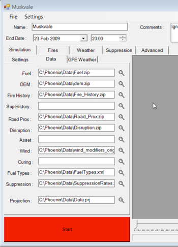
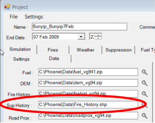
Simulation → Data
This is where you specify the location of all the input data files. The only data layer that must exist to run PHOENIX is the "Fuel" data layer, however all the other layers make the simulation more realistic. If there is no data file location specified, then the input value will be zero.
The "Weather" data location is specifically for the Gridded Forecast Weather. If none is specified, then the weather data stream specified in PHOENIX will be used. An additional option is for the times in the Gridded Forecast Weather to be all offset by a specified amount. For example, if it is known that the passage of a cold front is likely to be 3 hours earlier than the model predicted, you can put an offset value of 3 in the "Offset" box, if the cold front is slower than expected the offset might be -3.
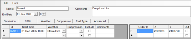
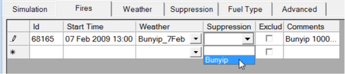
Simulation → Fires
This is where details about the location, ignition time, weather conditions and suppression options are specified.
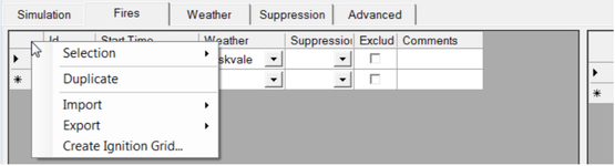
By right clicking in the left hand column of the fire list, a number of option menus appear. These are: Selection, Duplicate, Import, Export and Create Ignition Grid.
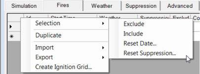
Under the "Selection" menu, there is an option to "Exclude" or "Include" all the selected fires in the simulation. This saves having to check or uncheck individual fires. Fires are selected by right clicking in the first (blank) column of the table. The use of the Shift and Ctrl keys in combination with the right mouse button works as it would in other applications when you select ranges or multiple records. There is also an option to change the "Start Time" and date for the selected fires. Again this global change saves times and reduces possible errors if large numbers of fires have to be altered.
Under the "Import" menu, there are options to import fire origins for an individual fire (in Lat, Long format), fire perimeters from existing fires (in CSV, KMZ, XML or SHP formats) or a list of fires (in CSV format).
Note: the coordinate system of the fire origin must be the same as the underlying data.
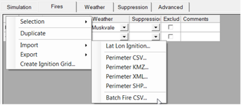
Using the "Export" menu, you can export a file (in Shapefile format) of ignition grid points that could be viewed in a GIS program.
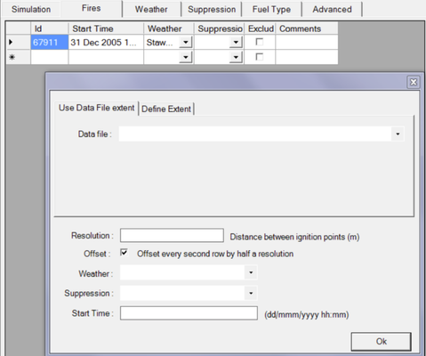
Finally, there is a tool that can be used to automatically create a uniform ignition grid for doing scenario testing or risk analysis. This ignition grid can be created within the extent of a specified Shapefile, or within an area defined by coordinates and grid spacing.
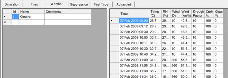
Simulation → Weather
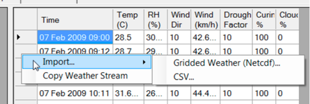
This is where a string of weather data can be specified. Values for the air Temperature (oC), Relative Humidity (%), Wind Direction (deg), Wind Speed (km/h), Drought Factor (0-10), Degree of grass Curing (%) and Cloud Cover (%) for specified times need to be made. The more frequent the time interval the better, but hourly data is good especially if it is supplemented with the times of key weather changes such as wind direction changes. PHOENIX linearly interpolates the weather values for times in between two time steps.
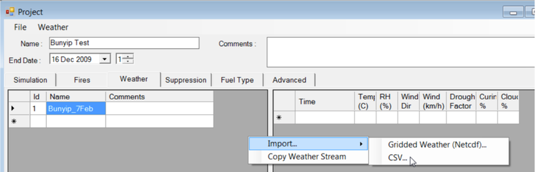
Weather data can be imported to PHOENIX from an MS-Excel spreadsheet or from a Gridded Weather file. This can be achieved by right clicking in the weather window to open the "Import" menu.
An alternative is to copy and save a weather stream that has been sourced from the Gridded Weather files. This is the second menu option.
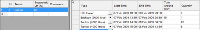
Simulation → Suppression
This tab allows you to specify the type and number of fire suppression resources to be applied to a fire. This may come from a previous project or can be built up from scratch.
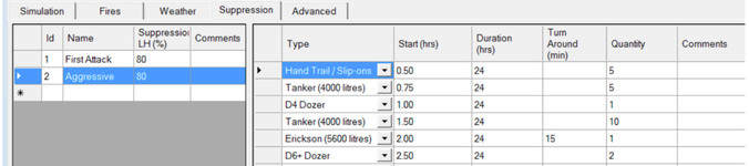
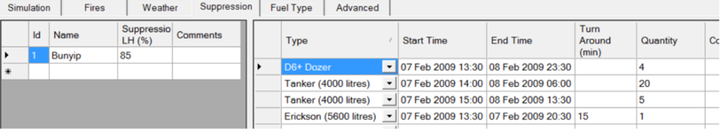
A suppression scenario can be built up by selecting one of the fire suppression resource types from the drop-down menu and then specifying the time it will be ready to start work on the fire edge, when it will be rested, and how many units of this resource time to use. The "Turn Around" time is only relevant to aircraft and refers to the time taken between drops of water, foam or retardant.
It is assumed that the suppression resources will work together and that they will start work at the origin (back) of the fire and work along the flanks moving forward. You have to specify what proportion of the suppression resources will be allocated to the left-hand flank and right-hand flank. This will depend on your fire suppression strategy. If a south-westerly wind change is forecast, then the majority of the suppression resources will usually be deployed to the left-hand (eastern) flank to reduce the blow out after the wind change.
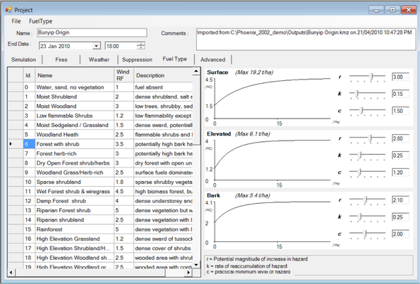
Simulation → Fuel Type
This sets out the fuel types and the expected fuel accumulation rates following fire. These parameters should not be changed unless you have very good reason to. All fuels are assumed to reaccumulate according to a exponential curve. The rate and peaks of accumulations can be altered for each fuel type. Beware - there are no default settings, so any changes become the new values. The effect of each fuel type on reducing the wind speed is also included in this table. This is the ratio of the windspeed at 10 m in the open compared with 1.5m inside the fuel (e.g. forest). All these fuel characteristics are stored in the project file, so each project will have a separate fuel list.
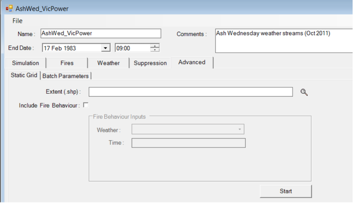
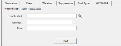
Simulation → Advanced
This is intended only for more advanced users with specialist knowledge. There are two main functions in this Tab - a "Hazard Map" feature and "Batch Parameters" feature already mentioned.
Hazard Map
This is to show a map of a specified area ("Extent") at a specified point in time. Running this model assumes the whole landscape is burning at the same (specified) time. So the output shows the potential fire characteristics for each cell across the landscape in terms of the potential fire intensity, flame height, fuel moisture ,etc. for the specific weather, fire history, fuel and topography relevant for the specified time. The output from this model must be viewed in a GIS.
My First Run

Exercise
This exercise will assume that you have already loaded the software and demonstration data onto the C: drive of your computer.
Assumptions
- you have the desired software stipulated in Set Up
- you have a picture viewer capable of viewing .png files
- the PHOENIX Rapidfire directory is C:\Phoenix\
Part 1 - Run an existing Project
- Step 1. Start PHOENIX RapidFire and Acknowledge the disclaimer
- Step 2. Open the demonstration project: File > Open database > C:\Phoenix\Projects\. In the Project menu find and open: "Bunyip_Bunyip7Feb.xml" (double click on project name).
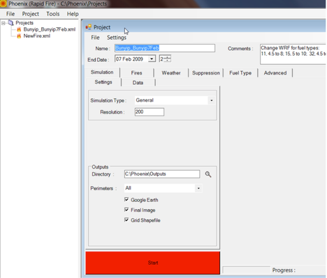
- Step 3. Do the following :
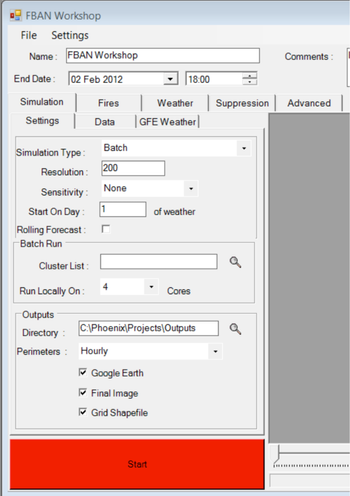
- Set the "Simulation Type" to "General" for a single fire simulation
- Set the "Resolution" to 200 metres
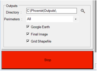
- Select "Perimeters" to "all"
- Check all three output options: "Google Earth", "Final Image" and "Grid Shapefile".
- Check to make sure the "Output Directory" and "Data Directories" are correct
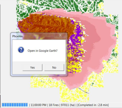
- Step 4. Select the big red "Start" button. After a short pause when the underlying data files are unzipped for use, an image showing the progress of the simulation should appear. An information bar at the bottom of the window indicates the relative progress, the time portrayed by the simulation, the number of fires running (original plus spotfires) and the progressive size of the fire. At the completion of the simulation (could take about 5 minutes) the computation time will be displayed and if a Google output has been specified, you will be asked if you wish to automatically display the output on Google. Select yes if possible.
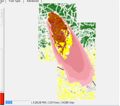
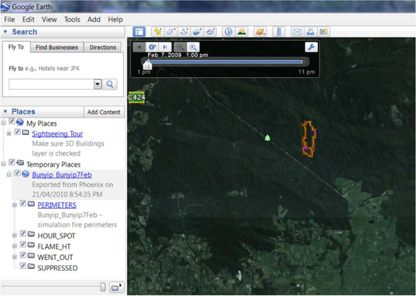
- Step 5. Display the output in Google Earth. Yellow and brown areas indicate the relative flame height, purple areas indicate cells where fires have entered, but self-extinguished, blue cells are cells effectively suppressed by firefighters, the shades of pink indicate ember density -darker pink indicating high ember density. The background colours show shades of green for relative amounts of forest or shrub fuels, shades of yellow show relative amounts of grassland fuels, grey cells show lines of fuel disruptions caused by roads, streams, or fire breaks of various types.
- Step 6. View output in Google Earth. The output is a "movie" and the control bar will be located in the top left corner of the viewing window. You can either drag the scrolling tab across the time bar or click on the play button to run the view automatically. In the tools on the movie bar, you can alter the play speed and the time reference. The output times from PHOENIX are in UTC time. If the times indicated on the movie bar look about 10 hours out, then UTC has not been selected.
Five fire characteristics are included in the Google output - "Perimeters" or isochrones, "Hour_Spot" which is the extent of potential spotfires, "Flame_Ht" which is the average flame height in each cell, "Went_Out" which indicates cells which started to burn but then self extinguished and finally, "Suppressed" which shows perimeter cells which have been extinguished by suppression forces. Each fire characteristic is in a separate layer and can be turned on or off.
Try viewing the output on Google Earth just showing the Flame Height and the Extent of Spotting. Try tilting, zooming and rotating the image to help understand the detail of the fire behaviour.
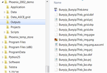
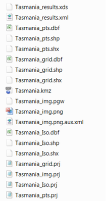
- Step 7. View the final fire image using a picture viewer or in a GIS. The .PNG images can be viewed alone or opened in a GIS. There are four types of output file stored: the KMZ file for viewing in Google Earth, the "GRID" shapefiles containing 27 input and output attributes for each grid cell, the IMG files which capture the final fire shape, and the ISOchrone files which show the progressive fire perimeters of the fire as it is modelled. The"GRID", "ISOchrone" and IMaGe files are best viewed in a GIS.
List of output files possible from the run of a single fire.
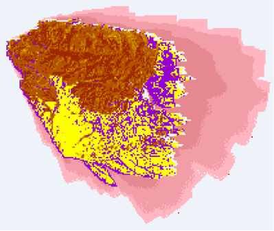
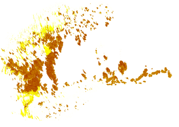
A PNG image file from a single fire.
- Step 8. Create a new project and explore the effect of changing modelling options on the outputs.
Part 2 - Create a New Project by Copying an Existing one
- Step 1. Open PHOENIX
- Step 2. Right click on the Bunyip project and select 'Copy' from the menu options
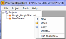
- Step 3. Give the copied project a new name such as 'Test'
- Step 4. Explore the effect of changing the resolution of the grid, alter the start and finish time of a fire, shift the ignition point of a fire, remove the fire history from the simulation, etc, etc. If you inadvertently corrupt the project, delete it and make another copy.
Part 3 - Create a New Project using 'Quick Start'
- Step 1. Open PHOENIX
- Step 2. From the Menu bar, select Project → New
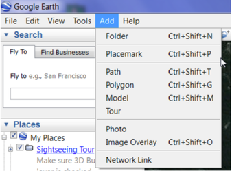
- Step 3. Enter an ignition location using a Latitude and Longitude location or create a place marker in Google Earth and point to the KMZ file for this place marker. In Google Earth, select the "Add" > "Placemark" option from the menu bar.
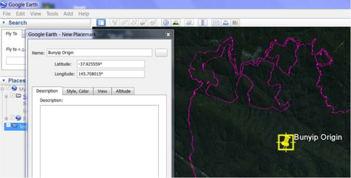
Insert a "Placemark" at the desired location and give it a name such as "Bunyip Origin". Save this placemark to your "Output" folder for PHOENIX. Then return to the "Quick Start" window and browse your way to the Placemark file in the "Output" folder.
- Step 4. Name the project, enter an ignition time to start the fire run, specify the duration of the fire run you want to model and then choose the gridded weather folder for the simulation. Note: you must make sure the start time and duration of the fire is within the range of the gridded weather data otherwise an error will occur when you select Go.
Part 4 - Create a New Project from Scratch
- Step 1. Copy the "New Fire" project template and name it appropriately, e.g. "Bunyip Test".
- Step 2. Open the project to input all the necessary details.
- Step 3. Set all the paths for the input and output files.
- Step 4. Select the Simulation Type (General) and Resolution (200m is good to start with).
- Step 5. In the "Fires" tab, enter the "Start Time" for the fire and then make sure the "End Date" falls an appropriate time after this. Enter the coordinates for the fire origin, these have to be in the same coordinate system as the underlying data which in this case is "Lamberts VicGrid GDA94". For the Bunyip fire, try the X, Y coordinates: 2561754, 2396979. You would normally need to get this information from a map, GPS or GIS.
- Step 6. Enter a stream of weather data from a spreadsheet or other table. The weather data must have eight (8) columns of data, in the correct format and order. The columns are: Time, Temperature, Relative Humidity, Wind Direction, Wind Speed (km/h), Drought Factor, Curing %, Cloud %. An example is given in the spreadsheet: "Bunyip_7Feb.xls". Note: make sure you get the format of the Date and Time correct. A cloud value of 0 means clear skies.
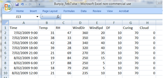
In the Weather tab, enter the name of the weather data (e.g. "Bunyip 7Feb") and then right click in the data window to bring up the "Import" option. Select the "CSV" format option. An "Import" window will open and here you can cut and paste the data from the spreadsheet into this import window.
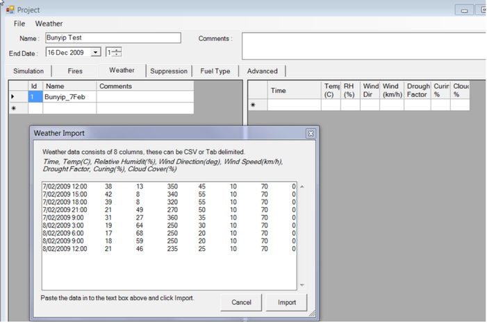
Providing all the data is in the correct format and you have the right number of columns, the data will be accepted in this window. Click the "Import" button on the bottom right corner to complete the process.
Check to make sure the start and finish times of the fire simulation are within the range of the weather data. The weather data needs to start 2 hours before the fire because a lag time is assumed in the model.
- Step 7. If you wish to have fire suppression effects included, now is the time to specify the type and number of suppression resources and when they will start work on the fire edge. Note: if you start the suppression effort before or at the same time as the fire, more than likely the fire will be suppressed before spreading, so don't be surprised if the model does not seem to run if you have suppression starting at or before the fire.
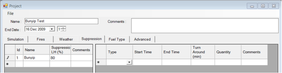
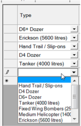
Start by giving the suppression effort a name. Then fill out the suppression details. Use the drop down list to choose a suppression type and then proceed to fill out the other details for each instance.
- Step 8. Run the model and view the output as done previously.
Questions to Address:
Q1 What is the modelled extent of the Bunyip fire on Black Saturday (7 Feb 2009) when the observed weather conditions and no effective suppression are included? Record the area burnt from Part 1 of this exercise.
A1Total Area Burnt (ha) [No suppression, Weather scenario ] |
|---|
Q2 What difference would it make to the extent of fire impact if you had 5 Erikson aircranes rather than just one? (Fire Suppression Scenario 2). Use the "Bunyip" suppression resources in one run of the model by adding in the "Fires" window. Record the area burnt. Then modify the suppression resources to include 5 Eriksons and run the model again. Record the area burnt this time. What difference does it make?
A2
Total Area Burnt (ha) [Suppression 1 Erikson, Weather scenario 1] | |
|---|---|
Total Area Burnt (ha) [Suppression 5 Eriksons, Weather scenario 1] |
Q3 What difference would it make to the extent of fire impact if you had have had a regular prescribed burning program in place in the Bunyip State Forest? (Fire History Scenario 2). Rerun the simulation as for Part 1, but this time include the supplementary fire history from the shapefile: "Fire History.shp" in the C:\Phoenix\Data folder.
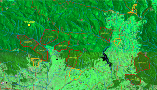
Created fire history layer. Labels refer to burn date, e.g. 20001103 = 3 Nov 2000.
A3
Total Area Burnt (ha) | |
|---|---|
Total Area Burnt (ha) |
Q4 What difference would it have made to the size of the fire if the wind speed was generally 15 km/h slower and the relative humidity 20% higher? (Weather Scenario 2). Use the Excel spreadsheet (Bunyip_Feb7.xlsx in the Outputs folder) to create a copy of the weather data, but subtract 15 from each wind speed and add 20 to each relative humidity. Import this new data into a new weather scenario as was done in Step 6 of Part 4 of this exercise.
A4
Total Area Burnt (ha) | |
|---|---|
Total Area Burnt (ha) |
Q5 What is the difference between weather scenario 1 and 2 in the fire intensity distribution if you were to look at the proportion of the area burnt with an intensity of: 0-3000, 3000- 10000, 10000-30000, >30000 kW/m ? Open the output file: Bunyip_Bunyip7Feb_grid.dbf in MS-Excel, immediately "Save As" an MS-Excel spreadsheet to avoid corrupting the original data. Create a histogram of the fire intensity data in classes listed above (you may need to "turn on" the "Add-Ins" > "Analysis Toolpak" in MS-Excel to get access to the Histogram and other functions). Repeat this for both weather scenarios so that you can answer the question.
A5
Fire Intensity Range (kW/m) | Weather Scenario 1 | Weather Scenario 1 |
|---|---|---|
< 3,000 | ||
3,000 - 10,000 | ||
10,000 - 30,000 | ||
> 30,000 |
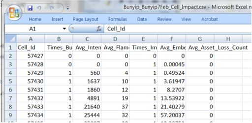
Q6 What is the difference to the level of impact on the Assets in the townships of Noojee, Neerim, Labertouche and Tonimbuk whether the prescribed burning existed or not and whether the weather was as severe as Black Saturday or the milder conditions used in Question 4 above? To answer these questions, you will need to run PHOENIX in the "Grid Analysis" simulation type. This will produce a set of output files, but the one of greatest interest here is: "Bunyip_Bunyip7Feb_Cell_Impact.csv" which can be opened and viewed in MS-Excel. This contains cell by cell details of the simulation including the asset impact. Compare the total asset loss for each of the weather and fire history situations addressed in this question.
A6
| Scenario | Asset Impact |
|---|---|
No Prescribed Burning 7 Feb 2009 Weather | |
No Prescribed Burning | |
With Prescribed Burning 7 Feb 2009 Weather | |
With Prescribed Burning |
Q7 What scenarios would you explore if you were interested in minimising the bushfire impact on Labertouche?
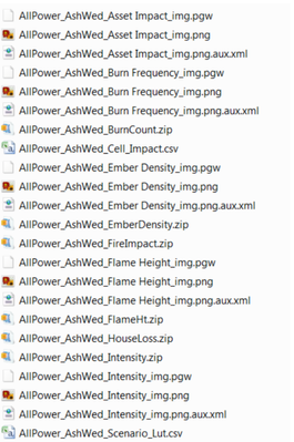
Appendix 1 - Output files from PHOENIX in 'GridAnalysis' simulation mode
List of files produced by PHOENIX RapidFire in 'GridAnalysis' mode.
Appendix 2 - Outputs from 'General' simulations
The outputs available will depend on what was selected in the simulation. They may include a shapefile of "perimeters" or "isochrones", a KMZ file to display on Google Earth, a PNG image and a shapefile of each grid cell impacted by the fire (and other cells on the same "tile" of data as the impacted cells).
| Files | Usage |
|---|---|
| XDS file | a diagnostic file showing the details of the simulation (technical use only) |
| XML file | contains all the results from the simulation, just in XML format |
| XXX_pts | contains all the results in a point shapefile where the point is the centroid of the cell |
| XXX_grid | contains all the results in a polygon (square) shapefile |
| KMZ | is the Google Earth file |
XXX_img | is the PNG format outputs |
XXX_iso | is the isochrone line in shapefile format if you want to see the progression of the fire as time contours |
Types of Output
PNG nad PGW files
'png' picture format can be displayed in GIS or a presentation or document
An image file of each major output from the simulations is produced as a PNG file. These images can be viewed with most image viewers and it can be displayed in a GIS when used with the associated "world" file (PGW).
The PNG images produced are:
Asset Impact (average)
Burn Frequency (number of times burnt)
Ember Density (average per unit area)
Flame Height (average maximum per fire)
Intensity (average maximum per fire)
An example of a png file:
ASC files
The ASCII files are quite large, so they have been compressed and have a ZIP suffix. These files are in an ASCII grid format and can be viewed in a GIS. These files contain the numeric value for each cell burnt and so can be displayed and manipulated in a GIS.
"BurnCount.zip", "EmberDensity.zip", "FlameHt.zip", "Houseloss.zip", "Intensity.zip" are all ASCII grid files of the same information used in the "png" files, but can be displayed in a GIS with full resolution and can be manipulated in the GIS if desired.
XML files
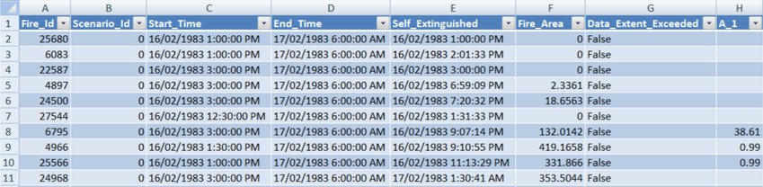
"FireImpact.zip" is a compressed "xml" format file that contains all the summary data from the ignition grid that covers the State. This includes the house impact data. The XML file can be converted to a CSV file in MS-Excel or MS-Access.
"Fire_Id" can be used to join this output with the "IgnGrid" (ignition grid or fire) layer in the GIS
CSV files
CSV are comma separated value files.
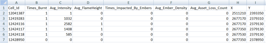
"Cell_Impact.csv" contains a summary of all the summary data from the data grid that covers the State. This includes the Cell_Id, number of times fire entered the cell "Times_Burnt", the average fireline intensity for all fires entering the cell "Avg_Intensity", the average flame height for all fires entering the cell "Avg_FlameHeight", the number of times embers impacted on the cell "Times_Impacted_By_Embers", the average density of embers in the cell for all impacts "Avg_Ember_Density", and the average number of assets lost for all fires impacting on the cell "Avg_Asset_Loss_Count" as well as the X and Y coordinate for the centroid of the cell.
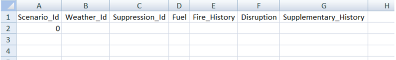
"Scenario_Lut.csv" contains a summary of all the simulation weather/suppression/fire history scenarios. In the power distribution network exercise, there is only one scenario so this file is not helpful.
Supplementary Data
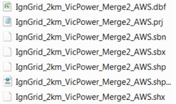
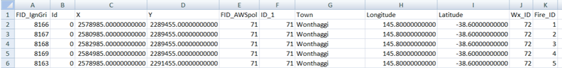
IgnGrid
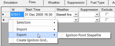
This is a shapefile of all the fire ignition points. The common field in this file is called "Fire_Id" which can be joined to the field of the same name is the "FireImpact.zip" file.
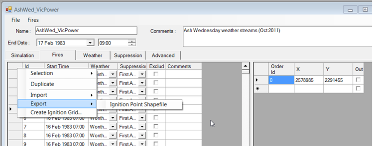
If the "IgnGrid" file does not already exist, you can create one in PHOENIX by exporting the "Fires" table. Right click on the table, choose "Export" and select "Ignition Point Shapefile" and the file will be created.
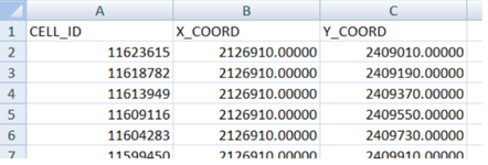
'Sg' or 'StaticGrid'
This is a shapefile, produced by PHOENIX's "Hazard" function, which is all the square polygons used for the input and output data in the simulation. The field "Cell_Id" is a common field in this shapefile and in the "Cell_Impact.csv" file.
This file could also be used to produce a set of centroid points for density analysis and the like.
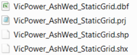
An empty grid can be produced with PHOENIX using the Advanced > Static Grid tabs with a suitable "Extent" shapefile such as the outline of the State (see figure below). If the "Include Fire Behaviour" box is not ticked, then an empty grid will be produced. The ID of the cells will be the same as for the outputs from the simulations.